1. Preprocessing

1.0 Introducing scprep

Scprep is a lightweight scRNA-seq toolkit for Python Data Scientists

Most scRNA-seq toolkits are written in R, but we develop our tools in Python. Currently, Scanpy is the most popular toolkit for scRNA-seq analysis in Python. In fact, if you’d prefer to use that, you can find most of our lab’s analytical methods including PHATE and MAGIC in scanpy. However, scanpy has a highly structured framework for data representation and a steep learning curve that is unnescessary for users already comfortable with the suite of methods available in Pandas, Scipy, and Sklearn.

To accomodate these users (including ourselves) we developed scprep (Single Cell PREParation). scprep makes it easier to use the Pandas / Scipy / Sklearn ecosystem for scRNA-seq analysis. Most of scprep is composed of helper functions to perform tasks common to single cell data like loading counts matrices, filtering & normalizing cells by library size, and calculating common statistics. The key advantage of scprep is that data can be stored in Pandas DataFrames, Numpy arrays, Scipy Sparse Matices, it is just works.

For users starting out, you might find it more valuable to spend time spent getting comfortable with these tools because they can be used for analysis of all kinds of data, not just scRNA-seq. If you want to learn more, checkout the Numpy Quickstart Tutorial, the Pandas Tutorials, the Matplotlib Tutorials, and consider getting a copy of Wes McKinney’s book Python for Data Analysis. McKinney is the original author of Pandas, and I’m glad I went through the book at the beginning of my PhD.

Installation

From here on out, I will assume that you have Python, Numpy, Pandas, Scipy, Scikit-learn, and Matplotlib all installed.

The scprep package is available on GitHub and on PyPI so the install is straightforward:

$ pip install --user scprep

In scprep you’ll find tools for loading single cell data (scprep.io), library size normalization (scprep.normalize), transforming data (scprep.transform), performing statistical calculations (scprep.stats), and many others. Check out the screp documentation for the full API.

1.1 - Using scprep to load a 10X Genomics counts matrix

Most of the labs we work with use 10X Genomics for single cell sequencing, so we’ll use this as an example.

Say your 10X data is in /home/user/data/my_sample. To load your data, run:

import scprep
data_uf = scprep.io.load_10X('/home/user/data/my_sample/outs/filtered_gene_bc_matrices/my_genome/', sparse=True, gene_labels='both')

Here, data_uf is my shorthand for ‘data_unfiltered’. load_10X and other scprep.io functions return a Pandas SparseDataFrame by default. The SparseDataFrame behaves similarly to regular Pandas DataFrames, but take up much less memory by storing only non-zero values and their indices in memory. Note: operations are sparse matrices are slower than dense matrices. If you can afford to store the dense matrix in memory, set sparse=False.

As an aside, many genome annotations (the descriptions of where genes are located on a given genome) contain non-unique gene symbols, so with gene_labels=both we store the gene symbol and the gene ID as 'ACTB (ENSG00000075624)'.

If you look at the head of your data, you should see something like this:

data_uf.head()

[sparse_dataframe_head.png]

Now, let’s start preprocessing your data.

1.2 - Merging batches using scprep (optional)

This is the point to merge batches if you have multiple samples from the sample experiment that you want to compare. Although we’ll talk briefly about batch effects later, we’ll write a whole post about how to correct them at another point.

How to combine samples

Here, what we’re doing is taking counts matrices from each sample and stacking them vertically. We’ve implemented this in the scprep.utils.combine_batches function.

For this example, I’m going to use the Embryoid Body timecourse covered in the PHATE tutorial.

Two important notes:

First, it’s important to know exactly which rows of the data matrix correspond to which sample so that we can separate them during downstream analysis. To facilitate this, combine_batches() takes an list batch_labels that contains one label per sample and returns an array sample labels that contains the sample label for each row in the resulting matrix.

Second, it’s possible (and exceedingly common) for the same cell barcode to appear in multiple experiments. This becomes an issue when combining batches because you want each row to have a unique index. To solve this problem, we append the sample label to the cell barcode by setting append_to_cell_names=True. This turns cell barcode AAACATACCAGAGG-1 from sample Day0-3 to AAACATACCAGAGG-1_Day0-3

# Loading each of 5 timepoints
T1 = scprep.io.load_10X(os.path.join(download_path, "scRNAseq", "T0_1A"), gene_labels='both')
T2 = scprep.io.load_10X(os.path.join(download_path, "scRNAseq", "T2_3B"), gene_labels='both')
T3 = scprep.io.load_10X(os.path.join(download_path, "scRNAseq", "T4_5C"), gene_labels='both')
T4 = scprep.io.load_10X(os.path.join(download_path, "scRNAseq", "T6_7D"), gene_labels='both')
T5 = scprep.io.load_10X(os.path.join(download_path, "scRNAseq", "T8_9E"), gene_labels='both')

# Concatenating data matrices
EBT_counts, sample_labels = scprep.utils.combine_batches(
    data=[T1, T2, T3, T4, T5],
    batch_labels=["Day0-3", "Day6-9", "Day12-15", "Day18-21", "Day24-27"],
    append_to_cell_names=True
)

# remove objects from memory
del T1, T2, T3, T4, T5  

1.3 - Filtering cells by library size

Why we filter cells by library size

In scRNA-seq the library size of a cell is the number of unique mRNA molecules detected in that cell. These unique molecules are identified using a random barcode incorporated during the first round of reverse transcription. This barcode is called a Unique Molecule Indicator, and often we refer to the number unique mRNAs in a cell as the number of UMIs. To read more about UMIs, Smith et al. (2017) write about how sequencing errors and PCR amplification errors lead to innaccurate quantification of UMIs/cell.

Depending on the method of scRNA-seq, the amount of library size filtering done can vary. The 10X Genomics CellRanger tool, the DropSeq and InDrops pipelines, and the Umitools package each have their own method and cutoff for determining real cells from empty droplets. You can take these methods at face value or set some manual cutoffs based on your data.

Visualing the library size distribution using scprep

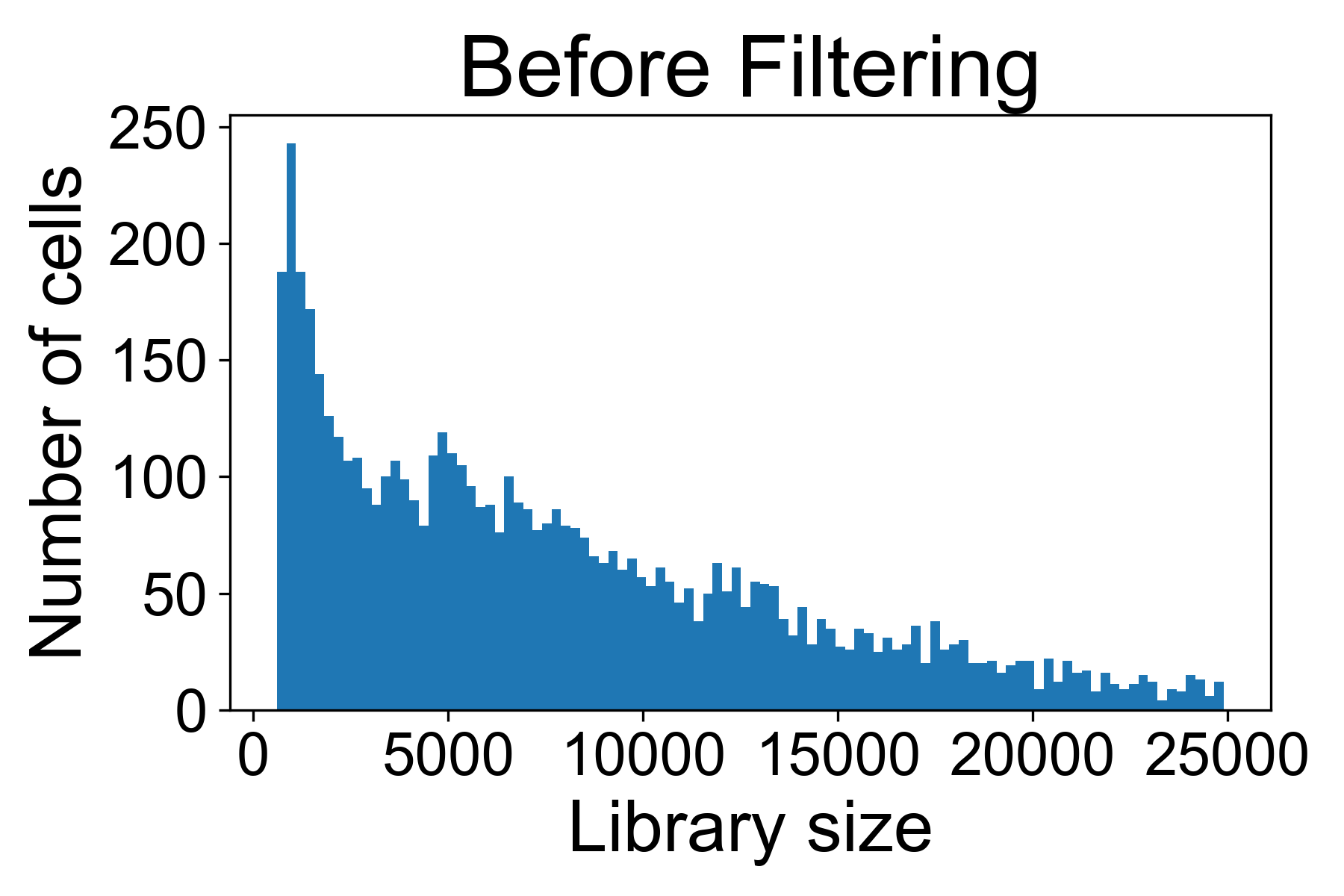
There is a helper function for plotting library size from a gene expression matrix in scprep called scprep.plot.plot_library_size().

Here we can see a typical library size for a 10X dataset from Datlinger et al. (2017). In this sample we see that there is a long tail of cells that have very high library sizes.

Selecting a cutoff

Several papers describe strategies for picking a maximum and minimum threshold that can be found with a quick google search for “library size threshold single cell RNA seq”.

Most of these pick an arbitrary measure such as a certain number of deviations below or above the mean or median library size. We find that spending too much time worrying about the exact threshold is inefficient.

For the above dataset, I would remove all cells with more than 25,000 UMI / cell in fear they might represent doublets of cells. I will generally also remove all cells with fewer than 500 reads per cell.

Filtering cells by library size

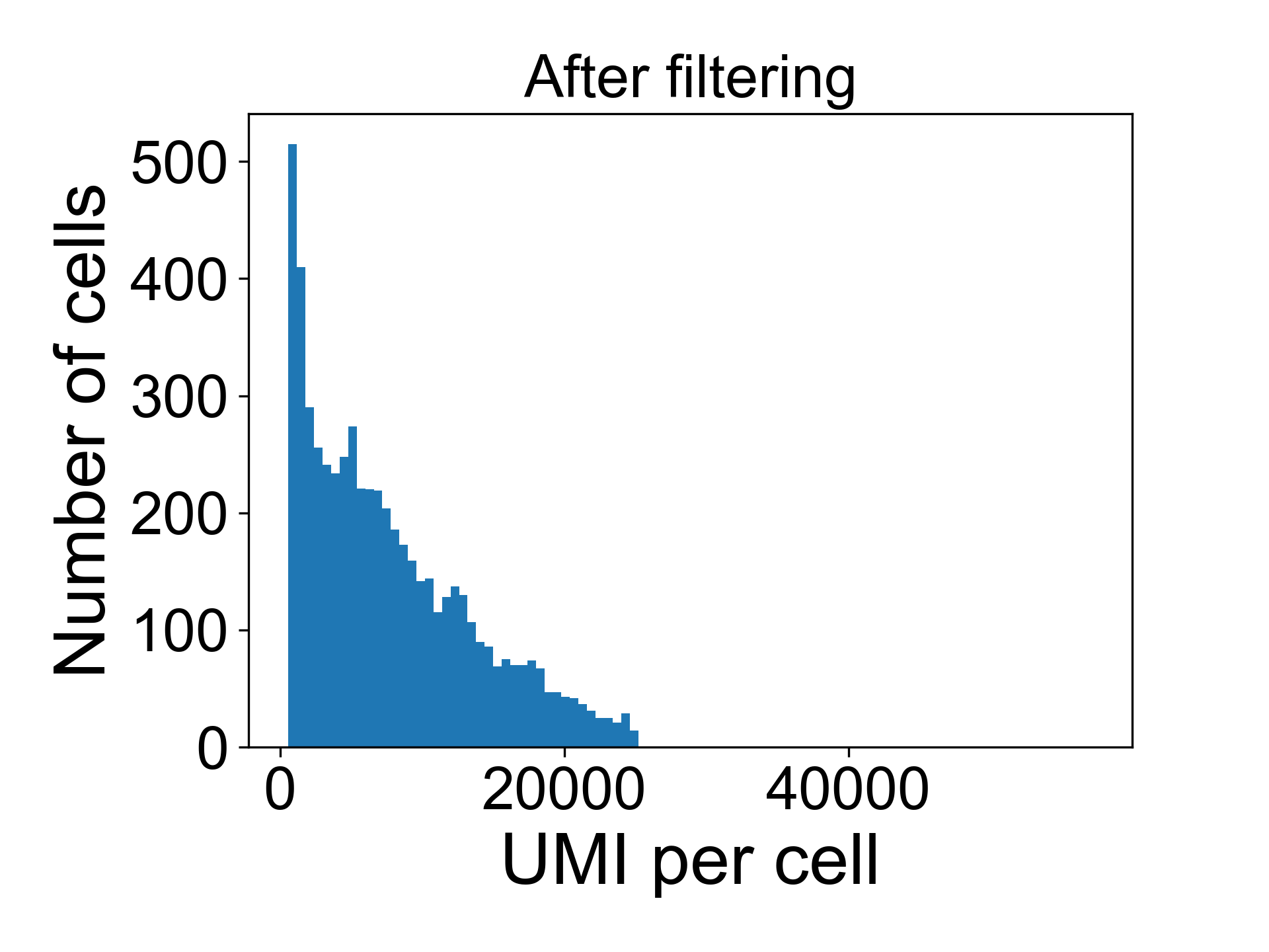
You can do this using scprep.filter.filter_library_size(). The syntax looks like:

data = scprep.filter.filter_library_size(data_uf, cutoff=25000, keep_cells='below')

And now when we plot the library size we see:

Note that there are many different valid distributions of library sizes. See the following three libraries, all generated from different tissues in the zebrafish embryo. One of the libraries is from a failed experiment, and the other two are from published papers.

Can you tell which is which?

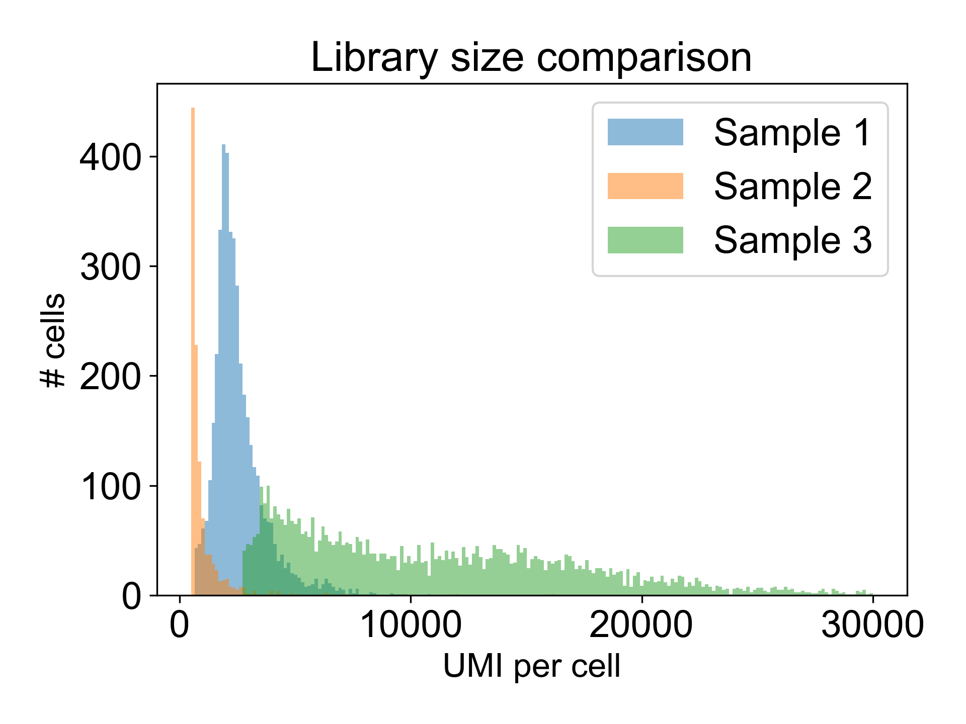
Here, Sample 1 is from Pandley et al. (2018), Sample 2 is an internal failed experiment, and Sample 3 is from Farrell et al. (2018). The low library size in Sample 2 is the giveaway with 90% of cells having fewer than 1200 UMI/cell and a mode at 325 UMI/cell. Additionally, this library generated a Low Fraction Reads in Cells alert in the Cell Ranger web summary with only 33% of reads assigned to cells. To learn more about what this means, read this post in the 10X Forums..

1.4 - Filtering lowly expressed genes

Why remove lowly expressed genes?

Capturing RNA from single cells is a noisy process. The first round of reverse transcription is done in the presence of cell lysate. This results in capture of only 10-40% of the mRNA molecules in a cell leading to a phenomenon called dropout where some lowly expressed genes are not detected in cells in which they are expressed [1, 2, 3, 4]. As a result, some genes are so lowly expressed (or expressed not at all) that we do not have sufficient observations of that gene to make any inferences on its expression.

Lowly expressed genes that may only be represented by a handful of mRNAs may not appear in a given dataset. Others might only be present in a small number of cells. Because we lack sufficient information about these genes, we remove lowly expressed genes from the gene expression matrix during preprocessing. Typically, if a gene is detected in fewer than 5 or 10 cells, it gets removed.

Here, we can see that in the T cell dataset from Datlinger et al. (2017), there are many genes that are detected in very few cells.

genes_per_cell = np.sum(t_cell_data > 0, axis=0)

fig, ax = plt.subplots(1, figsize=(4,6))
ax.hist(genes_per_cell, bins=100)
ax.set_xlabel('# cells in which gene is expressed')
ax.set_ylabel('# of genes')
ax.set_yscale('symlog')
ax.set_title('Gene detection across cells')
fig.tight_layout()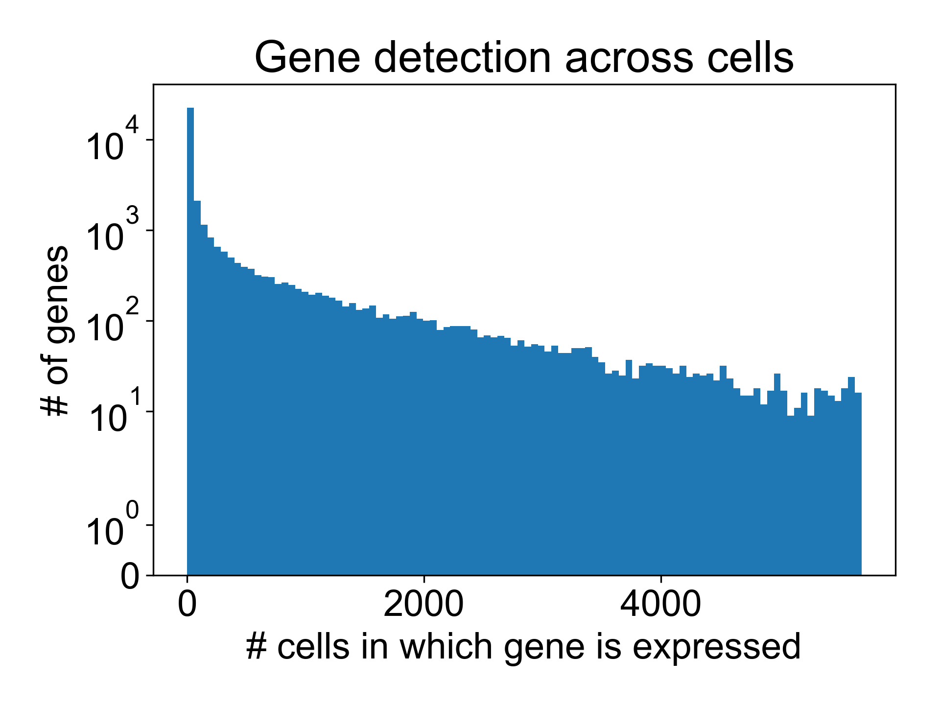

Here, around 16,000/35,000 genes are detected in fewer than 10 cells. We can remove these columns from the gene expression matrix moving forward.

How to remove lowly expressed genes using scprep.

The syntax to remove these genes is similar to filtering on library size. The scprep function is scprep.filter.remove_rare_genes(). You can use it like this:

data = scprep.filter.remove_rare_genes(data, cutoff=0, min_cells=5)

Another advantage of removing rare genes from our counts matrix is that it reduces the dimensions of the matrix that we’re working with. Instead of needing to do computations over a matrix that is 10,000x35,000, we are now working with one that is 10,000x16,000.

1.5 - Library size normalization

Why library size normalize?

Now that we have our cells filtered by library size and have removed lowly expressed genes from our dataset, it’s time to normalize the data. Library size normalization is meant to align the scales of gene expression across cells that have different # of UMIs / cell. This is equivalent to comparing only the ratios of genes detected within a cell as opposed to comparing the absolute quantity of each RNA.

Mathematically, this process involves diving the count of each gene in each cell by the # UMIs in that cell. Optionally, one may then multiply the gene expression in all cells by a constant, such as the median # UMIs /cell in an experiment. This is purely a stylistic choice, but makes interpreting gene expression values a little easier.

Normalizing library size using scprep

This step is accomplished using the scprep.normalize.library_size_normalize() function with the following syntax:

data_ln = scprep.normalize.library_size_normalize(data)

Here, I use data_ln to refer to data that has been library size normalized.

1.6 - Removing cells with high mitochondrial gene expression

What does high mitochondrial gene expression indicate?

Generally, we assume that cells with high detection of mitochondrial RNAs have undergone degradation of the mitochondrial membrane as a result of apoptosis. This may be from stress during dissociation, culture, or really anywhere in the experimental pipeline. As with the high and low library size cells, we want to remove the long tail from the distribution. In a successful experiment, it’s typical for 5-10% of the cells to have this apoptotic signature.

Plotting mitochondrial expression

Let’s look at the mitochondrial expression from Datlinger et al. (2017). Here, the dashed line is the 95th percentile of mitochondrial expression.

# get mitochondrial genes
mitochondrial_gene_list = np.array([g.startswith('MT-') for g in data_ln.columns])

# get expression
mito_exp = data_ln.loc[:,mitochondrial_gene_list].mean(axis=1)

# plotting
fig, ax = plt.subplots(1, figsize=(6,5))

ax.hist(mito_exp, bins=100)
ax.axvline(np.percentile(mito_exp, 95))
ax.set_xlabel('Mean mitochondrial expression')
ax.set_ylabel('# of cells')
ax.set_title('Mitochondrial expression')

fig.tight_layout()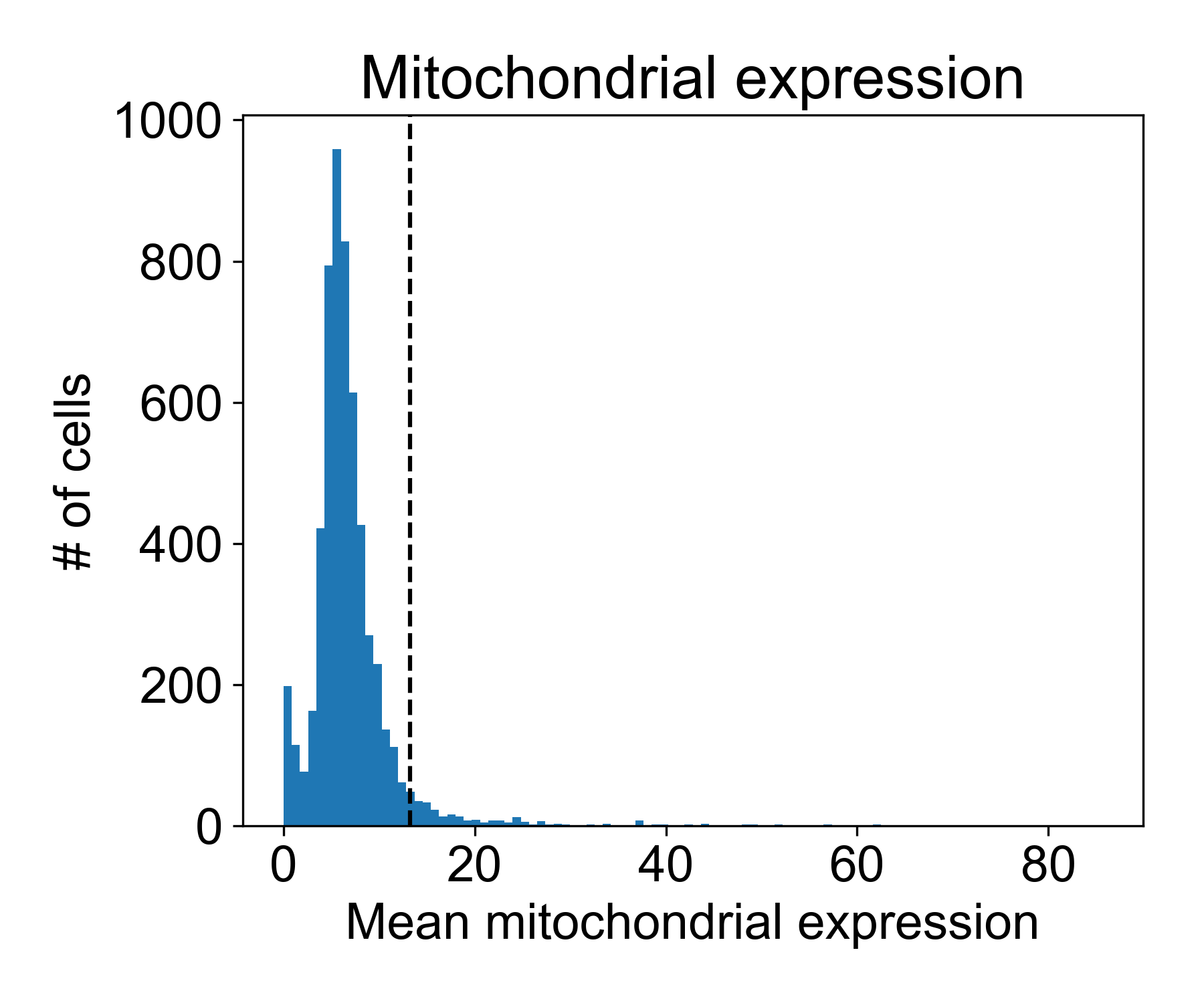

Removing cells with high mitochondrial expression using scprep

Each genome and species will have its own list of mitochondrial genes and associated symbols. In human and mouse, these genes start with ‘MT-’. However, as there’s no standard, we didn’t want to include a function for filtering mitochondrial expression directly in scprep. Instead, we provide the scprep.filter.filter_values() function. This method takes data and an array values and removes all cells from data where values is above or below the set threshold.

Here, this would look like:

# filter cells above 95th percentile
data_ln = scprep.filter.filter_values(data_ln, mito_expression, percentile=95, keep_cells='below')

1.7 - Transforming data

Our final step for preprocessing is to transform the data so that it’s usable for the algorithms that we’re using later.

The purpose of transforming data is to make sure that each gene or feature in our counts matrix is counted equally. Because of math, if we’re doing something like calculating the Euclidean distance between two cells, genes that are more highly expressed (i.e. have larger values) will be considered more important.

There are many transforms, but the two most common for scRNA-seq are the log-transform and the square-root transform. In CyTOF, the arcsinh transform is also popular. You can access all of these using scprep.transform.log(), scprep.transform.sqrt() or scprep.transform.arcsinh().

One note: the log-transform doesn’t like zeros, which are incredibly common in single cell datasets. To overcome this, people commonly add a pseudocount to their data, either 1 or a very small value called machine epsilon. Personally, I don’t like this because it skews the relationships between small values, which are a huge portion of single cell counts matrices.

Instead, we use the squareroot transform 99% of the time. The syntax couldn’t be simpler:

data_sq = scprep.transform.sqrt(data_ln)

We’re done preprocessing!

Congratulations, we’re ready to start visualizing!