Part 1: The problem
Single cell RNA-sequencing (scRNA-seq) is an increasingly popular method for measuring transcriptome-wide gene expression in single cells. However, there are several technical challenges that make analysing scRNA-seq data difficult. One of the biggest hurdles stems from the fact that of the roughly 100,000-300,000 mRNAs in a cell, only 10-40% are captured using current scRNA-seq protocols [1], [2], [3], [4]. As a result, all genes in all cells are undercounted, and lowly expressed genes may be recorded at 0s in the gene expression matrix despite being expressed.
This undercounting adds several hurdles to the analysis of scRNA-seq data that do not exist for bulk-RNA sequencing. In this post, we will first discuss a few of these hurdles (in part 1) and then how they can be addressed using MAGIC (in part 2), our recently published data denoising and imputation method.
In part 1 we will discuss the following:
Why are molecules undersampled in scRNA-seq?
How does undercounting/dropout obscure biology?
How can imputation solve these problems?
RT inefficiency leads to undercounting genes and “dropout”
As we mentioned above, only 10-40% of the transcripts in a given cell are captured in current scRNA-seq methods. For the most part, this is because doing the first round of reverse transcription (RT) and subsequent PCR amplification in the presence of cell lysate in nanoliter droplets is not very efficient. As a result, it’s better to think of scRNA-seq as a sampling method, as opposed to bulk RNA-sequencing which is more akin to a census or counting method.
In the MAGIC paper, we showed what this looks like. It’s hard to establish a “ground truth” for single cell data, so we picked a large bulk C. elegans time course and simulated a 20% mRNA capture efficiency by down-sampling molecules in the dataset. On the left is the original data for 9861 genes in 206 worms, and the right is the simulated undercounted data.
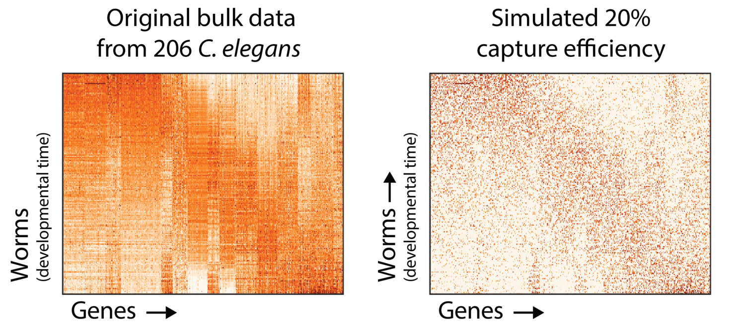
As you can see, there are a lot of zero values. The question is, are some zeros different from others?
When reading about scRNA-seq, it’s difficult to avoid the word “dropout.” It’s even harder to find a consistent definition of the term. The most common definition we’ve come across refers to when a gene is lowly expressed, say in the range of 1-20 molecules / cell. Now if you’re only capturing 10% of all molecules in a cell, and assume this sampling follows a negative binomial distribution, you will find that in many cells 0 unique reads will be observed despite the gene being expressed. This “observed as 0, but present” is termed dropout or a technical zero. This is opposed to a gene that just isn’t expressed in that cell, which is called a true or biological zero.
We will get more into this later, but we think it’s a bad idea to think about dropout as a problem only affecting lowly expressed genes because undercounting happens to all genes regardless of expression. It just so happens that for lowly expressed genes, undercounting leads to an observation of 0. This is fundamentally different from a problem where there are missing values that might be recorded as 0, such as the Netflix Problem. In the case of missing values, you know what you don’t know, and there exist very efficient and elegant methods to solve this problem, such as nuclear norm matrix completion. With scRNA-seq, we’re dealing with unknown unknowns.
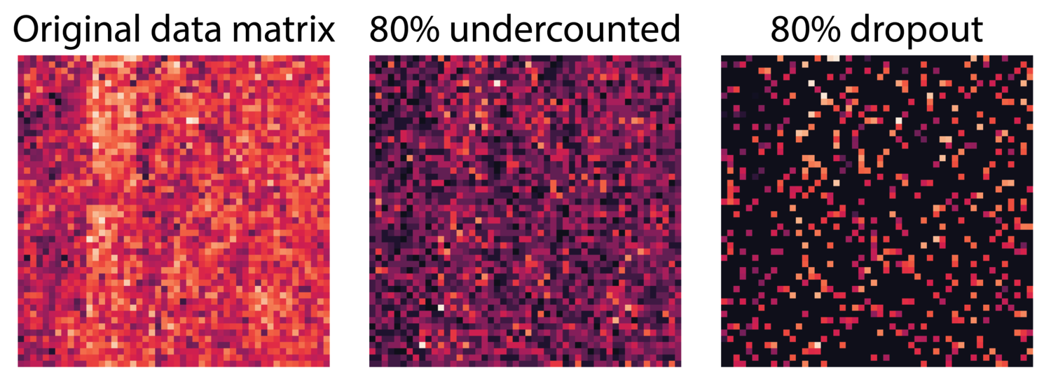
To illustrate this, see the three matrices below. The left is the original data matrix, the middle matrix is undercounted, i.e. 80% of the molecules are not counted so values are undercounted, in the third matrix 80% of the entries are set to zero. In scRNA-seq, undercounting produces a gene expression matrix more like the middle matrix where every entry can be affected.
There are many complex processes that add noise to gene expression data in scRNA-seq. We would like to note here that MAGIC makes no attempt to explicitly model these processes or assume a particular data-generating distribution. Instead, MAGIC assumes that gene expression in scRNA-seq follows the smoothness assumption. That is, we assume that the close neighbors of a cell contain gene expression information that can be used to recover information lost to undercounting in that cell. We’ll discuss this further in part 2 of this post.
Undercounting RNA molecules obscures biology
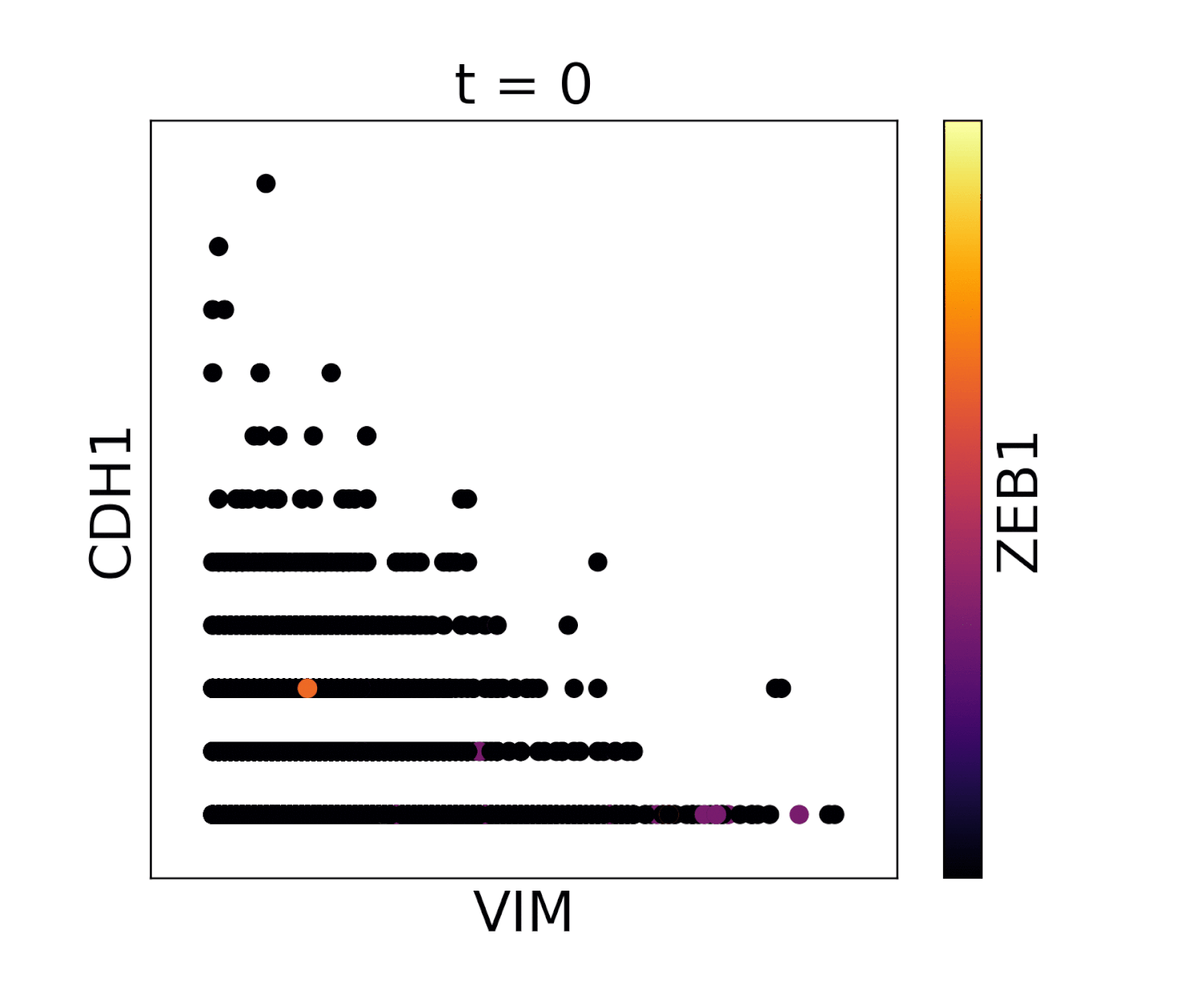
It’s not hard to imagine that dealing with data missing 90% of counts is a problem. Indeed, working with raw scRNA-seq data is a challenge - many biological signals are obscured and many types of analyses are impossible to do on sparse data. For example, dropout obscures gene-gene relationships. To illustrate this let’s look at the following two gene-gene scatterplots of an EMT dataset that we presented in the MAGIC paper:
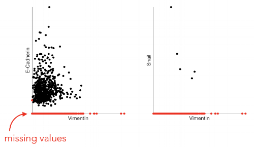
We expect Vimentin and E-Cadherin to be negatively correlated, since Vimentin is a mesenchymal marker and E-Cadherin is an epithelial marker. However, due to the undercounting, this relationship is not apparent. Similarly, we expect Vimentin and Snail to be positively correlated as Snail is a TF involved in regulation of the mesenchymal state.
How can we overcome undercounting?
Although we observe a small sample of mRNAs in a cell, many genes are redundant. Sets of transcription factors regulate modules of genes together. This means that the underlying gene expression state space is inherently low-dimensional and the feature set is not truly independent. However, we’re still left with the problem of figuring out how to use this inter-dependency of genes to recover undercounted gene expression.
Part 2: MAGIC
In part 1, we wrote about how technical challenges in scRNA-seq lead to a phenomenon that we’re calling undercounting. Because of inefficiencies in mRNA capture, the counts for all genes in each cell of a gene expression matrix represent a subsample of all mRNAs present in that cell. Here, we will introduce our solution to this problem, called MAGIC, and discuss its practical application to scRNA-seq data.
Specifically, we will discuss:
How MAGIC recovers gene expression lost to dropout
Interpretation of non-zero values after MAGIC
Selecting optimal diffusion time for MAGIC
Does MAGIC mix clusters?
Minimum cell numbers for MAGIC
Where does MAGIC fit in your pipeline
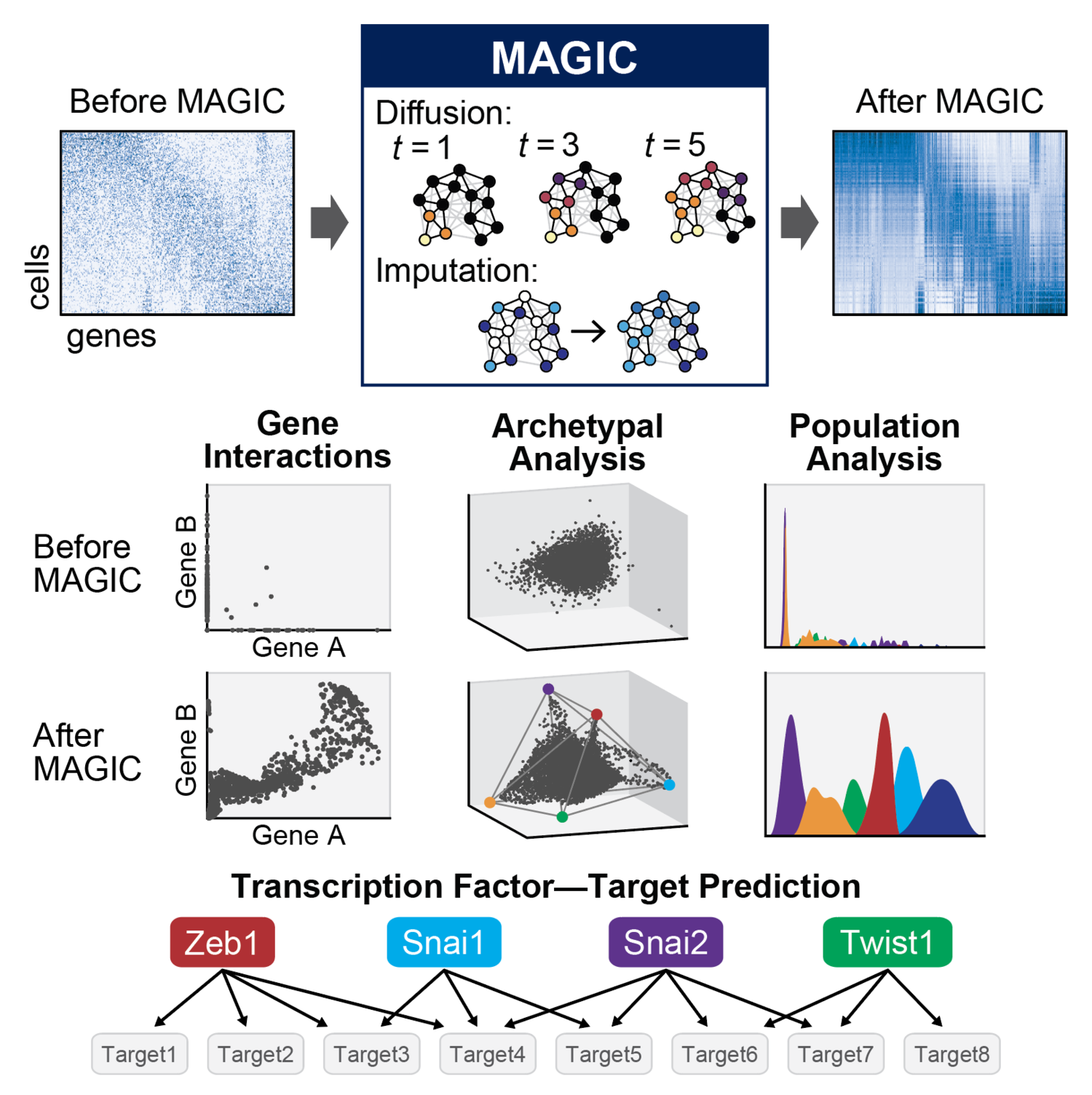
MAGIC
In our recent paper Recovering Gene Interactions from Single-Cell Data Using Data Diffusion, we propose a data imputation and denoising algorithm called MAGIC (Markov Affinity-based Graph Imputation of Cells). The idea of MAGIC is that we first learn the underlying structure, or manifold, of the data, and then recover the gene values using this manifold. To do this, MAGIC uses a cell-cell affinity graph to construct a Markov diffusion operator that is then used to diffuse data between cells, in the process filling in missing values and generally denoising the data.
Low-pass filter on the manifold
MAGIC has two parts: 1) learning the underlying structure, or manifold, of the data, and 2) imputing and denoising the gene counts by filtering them as signals on this manifold.
For part 1 we first compute a cell-cell Markov affinity matrix. This matrix is a diffusion operator and we can take powers of this operator to perform a random walk on the graph. This enables us to learn the manifold of the data without making any assumptions about its shape.
For part 2 we consider genes to be signals on the graph and we low-pass filter them by multiplying the powered diffusion operator with the genes. The result is a denoised and imputed data matrix.
Another way to look at this process is in terms of graph signal processing. Powering the operator effectively performs a low pass filter on the spectrum of the graph. In a future blog post we will go deeper into understanding this, but briefly this means that we are eliminating high frequency dimensions from the graph. Since high frequency is associated with noise, including dropout, this effectively denoises and imputes the data.
Dropout versus biological zeros
We often get the question: “Does MAGIC remove all zeros? Even if they’re actual biological zeros?” The answer is yes AND no! The reason is that MAGIC effectively computes a neighborhood (in a non-linear way and on the manifold) and then exchanges values between neighboring cells. If, for some gene, all the neighbors have zero value, then after diffusion (data exchange) the values will still be zero. In this case we can conclude that we were dealing with a ‘real’ biological zero. If some of the neighbors were non-zero for this gene, then after diffusion all cells in the neighborhood will end up with a non-zero value. In this case the zeros were due to dropout. However, there is one caveat. In practice, due to the many steps of diffusion, it can be that after diffusion we end up with a small but non-zero value. One could naively interpret this as a non-biological zero that was due to dropout. This is not the case, and small non-zero values are still effectively biological zeros. Therefore, we recommend to not (only) look at the absolute values after imputation, but also at the relative values or distributions. In the figure below we show an example where after MAGIC there is a population of cells that, while not absolutely zero, effectively has no expression for the gene.
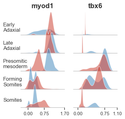
In the above figure we can see gene expression after magic in five cell types of the zebrafish embryo from Wagner et al (2018). In red is gene expression of cells from embryos in which chordin was knocked out using Cas9. In blue is the expression from control embryos. We can see that expression of myod1 is effectively 0 for some populations of cells in the forming somites and somites. Similarly, tbx6 is effectively note expressed in early or late adaxial cells. Although close inspection shows expression of these genes is slightly above 0, we can infer that this gene is not expressed in these cells.
Optimal diffusion time
In MAGIC we perform data diffusion by powering the Markov diffusion operator. The number of times we power, and thus number of steps we walk, is called the diffusion time and is denoted by the parameter t. The diffusion time controls the extent of the low pass filtering - the higher the t, the fewer eigenvectors are left. t is probably the most important parameter in MAGIC and should therefore be chosen carefully. In order to ensure an optimal value of t we provide (by default) an automatic method for picking it. This method is based on the idea that as we diffuse the data changes and that the rate of change of the data reflects what kind of signal we are altering. There are two types of signals in the data, the biological signal and the noise. The former is a low frequency signal and the latter a high frequency signal. As we diffuse, we first remove the high frequency noise and we observe a rapid change in the data. After a number of diffusion steps we enter the data (non-noise) regime and as a result the change in data is much slower. The goal is to set t to be right at this regime change, such that we have removed most noise but not the actual biologically meaningful signal. By quantifying the change in data (||data_t - data_t-1||) as a function of t we can find the regime change by picking t at the elbow point.
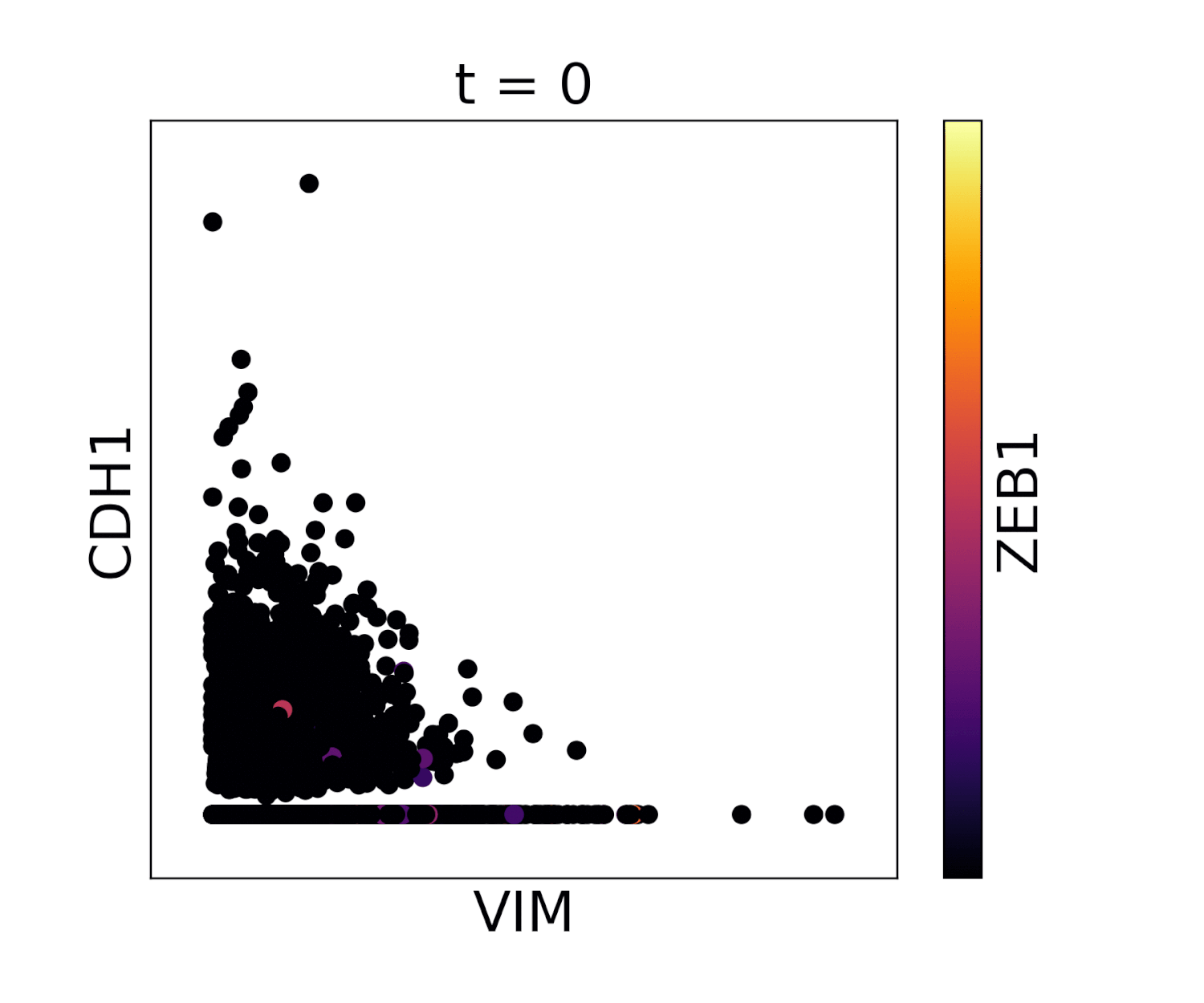 Visualization of cadherin, vimentin and zeb1 from the EMT dataset in the MAGIC paper.
Manual diffusion time
Our automatic diffusion time method is designed to pick a value of t that removes most of the noise but doesn’t remove much real biological signal. However, sometimes a user may want to do more diffusion for example when the data is especially noisy, and sacrifice some of the signal in return for more denoising. Conversely, a user may not want to sacrifice any biological signal and want less diffusion. In these cases we advise to first run automatic t selection and then manually choose a t that is slightly lower or higher.
In addition, it may just be that the automatically selected value for t does not look good on your data. In this case you can pick t manually by gradually increasing t (e.g. starting at t=3) and visually inspect if the structure of the data is recovered but that it is not over-smoothed. For example, you can look at some known gene-gene relationships, or at the PCA after MAGIC. In addition, in the case that rare cell populations are present in the data, you can inspect whether these populations still exist after MAGIC and have not disappeared by being ‘pulled in’ by MAGIC. While the right t is data dependent, we have found that for almost all datasets the optimal t is between 3 and 12.
Cluster mixing
Another question that we often get is: “Does MAGIC contaminate cell types? Does it mix clusters or cell states/types that shouldn’t be mixed?” The answer is no, assuming that MAGIC is used correctly. The reason is that MAGIC learns the underlying nonlinear manifold of the data. This is something we will cover in more detail in future blog posts, but for now this means that the diffusion process follows the shape of the data. Diffusion doesn’t just mix each cell with every other cell, but it follows the biologically meaningful neighborhood structure of the data. This means that, effectively, the diffusion won’t leave a cluster or cell type/state and won’t mix cells that are biologically significantly different.
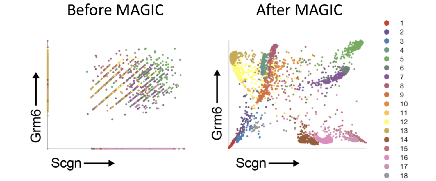
In the above figure we ran MAGIC on a mouse cortex dataset (Zeisel et al. 2015). We’re showing the relationship between two genes and the colors correspond to the clusters reported by the authors. We can see that MAGIC preserves the clusters and does not mix them.
Cell numbers
MAGIC requires a certain number of cells (data points) to work properly. Unfortunately we can’t give a specific number as this depends on the overall quality of the data, level of dropout and noise, and the underlying intrinsic dimensionality (effective degrees of freedom) of the data. In general, our experience is that at the very least we need 500 cells but more like 1000 for comfortable imputation. Moreover, the number of cells you have will determine the amount of detail that can be recovered. MAGIC may still work with 200 cells but would only recover one major trend in the data (e.g. a single progression). Including more cells enables recovery of more refined structures, e.g, additional branches or clusters.
Where to use MAGIC in your pipeline
MAGIC doesn’t just work on raw count matrices, fresh from your read mapping pipeline. MAGIC requires the data to be properly normalized and filtered. This preprocessing obviously depends on the data type and technology, but for single-cell RNA-seq data we have a set of preprocessing steps that work well and we recommend these to users of MAGIC. First, one has to make sure that “bad” cells are removed. For example, this can mean cells with small library size (total UMI). Next, the data has to be library size normalized, meaning that all values for a cell are divided by the total UMI in that cell. This prevents the neighborhoods from being dominated by cells of similar library size. Library size, generally, does not reflect biology since it is a result of the stochastic sampling of molecules. Next, we want to do a log type transform to the data. Popular is to take the natural log after adding a ‘pseudo’ count. The pseudo count enables taking log of zeros. A different, but similar, transform is the square root transform. This is what we often use. Like the log transform it effectively down weights highly expressed genes and high values, however it doesn’t require adding a pseudo count. After this filtering, normalization, and transform we can run MAGIC.
In the below animations we show the effect of library size normalization. Notice how the trends in the two gifs are essentially opposite - the first gif shows MAGIC applied to raw counts data, where the variation is driven exclusively by UMI count, giving a misleading representation of the data. The second gif, after library size and log normalization, reflects a gene-gene relationship which matches our understanding of these genes from the literature.
Without library size normalization:
With library size normalization:
Tutorials and help running MAGIC
We hope that with this post we have given you more insight into the workings of MAGIC and how to effectively use it. To learn how to use MAGIC we provide documentation and several tutorials in our Github directory. Additionally, we have a Slack group dedicated to helping users of our tools.